what’s new
in the tidyverse
in 2023?

🔗 mine.quarto.pub/tidyverse-2023

💻 github.com/mine-cetinkaya-rundel/tidyverse-2023

dr. mine çetinkaya-rundel

duke university + posit

2023-05-30

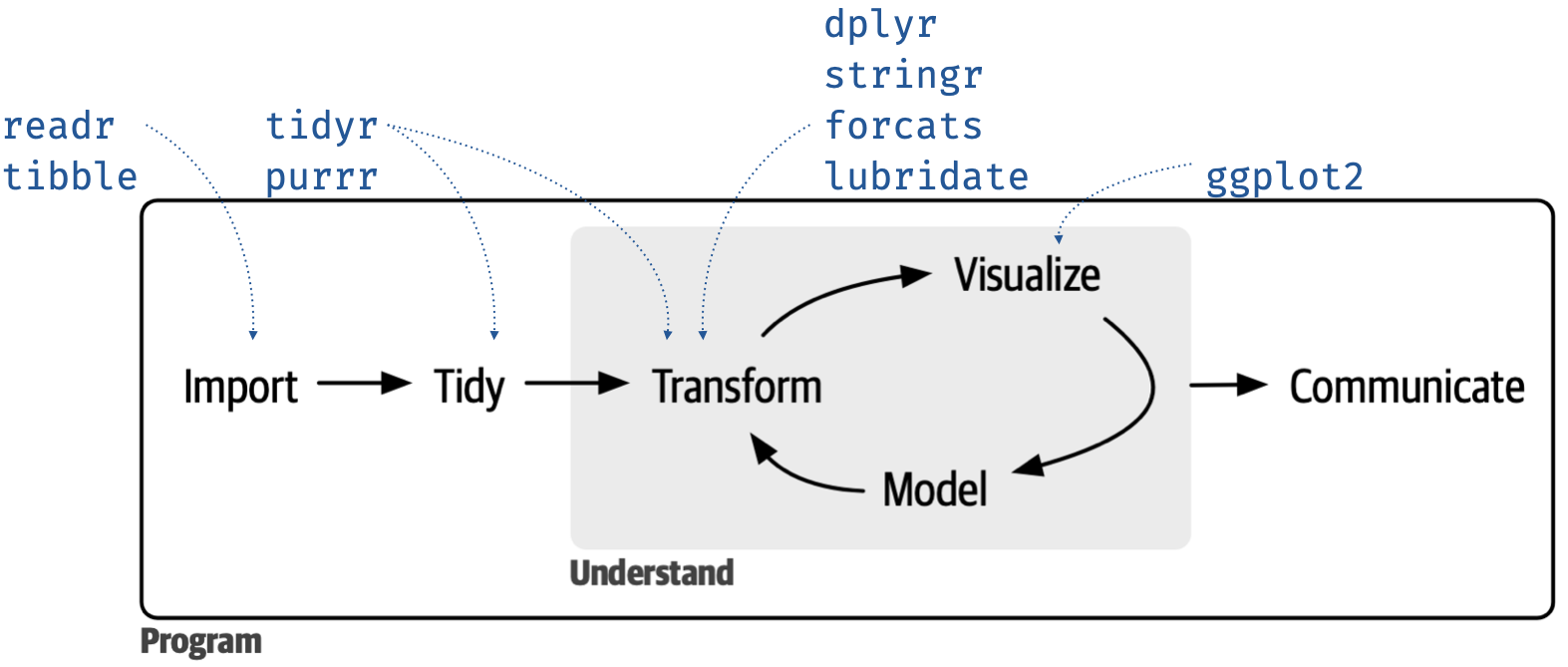
principles of the tidyverse

tidyverse

meta R package that loads nine core packages when invoked and also bundles numerous other packages that share a design philosophy, common grammar, and data structures

library(tidyverse)

── Attaching core tidyverse packages ──────── tidyverse 2.0.0 ──
✔ dplyr     1.1.2     ✔ readr     2.1.4
✔ forcats   1.0.0     ✔ stringr   1.5.0
✔ ggplot2   3.4.2     ✔ tibble    3.2.1
✔ lubridate 1.9.2     ✔ tidyr     1.3.0
✔ purrr     1.0.1
── Conflicts ────────────────────────── tidyverse_conflicts() ──
✖ dplyr::filter() masks stats::filter()
✖ dplyr::lag()    masks stats::lag()
ℹ Use the conflicted package to force all conflicts to become errors

tidyverse for data science

setup: penguins

library(palmerpenguins)
penguins

# A tibble: 344 × 8
  species island   bill_length_mm bill_depth_mm flipper_length_mm
  <fct>   <fct>             <dbl>         <dbl>             <int>
1 Adelie  Torgers…           39.1          18.7               181
2 Adelie  Torgers…           39.5          17.4               186
3 Adelie  Torgers…           40.3          18                 195
4 Adelie  Torgers…           NA            NA                  NA
5 Adelie  Torgers…           36.7          19.3               193
6 Adelie  Torgers…           39.3          20.6               190
# ℹ 338 more rows
# ℹ 3 more variables: body_mass_g <int>, sex <fct>, year <int>

a typical tidyverse pipeline

penguins |>
  drop_na(sex, body_mass_g) |>
  group_by(species, sex) |>
  summarize(mean_bw = mean(body_mass_g), .groups = "drop") |>
  ggplot(aes(x = species, y = mean_bw, fill = sex)) +
  geom_col(position = "dodge")

a typical tidyverse workflow

penguins |>
  group_by(species, sex) |>
  summarize(mean_bw = mean(body_mass_g))

`summarise()` has grouped output by 'species'. You can override
using the `.groups` argument.

# A tibble: 8 × 3
# Groups:   species [3]
  species   sex    mean_bw
  <fct>     <fct>    <dbl>
1 Adelie    female   3369.
2 Adelie    male     4043.
3 Adelie    <NA>       NA 
4 Chinstrap female   3527.
5 Chinstrap male     3939.
6 Gentoo    female   4680.
# ℹ 2 more rows

a typical tidyverse workflow

penguins |>
  drop_na(sex, body_mass_g) |>
  group_by(species, sex) |>
  summarize(mean_bw = mean(body_mass_g))

`summarise()` has grouped output by 'species'. You can override
using the `.groups` argument.

# A tibble: 6 × 3
# Groups:   species [3]
  species   sex    mean_bw
  <fct>     <fct>    <dbl>
1 Adelie    female   3369.
2 Adelie    male     4043.
3 Chinstrap female   3527.
4 Chinstrap male     3939.
5 Gentoo    female   4680.
6 Gentoo    male     5485.

a typical tidyverse workflow

penguins |>
  drop_na(sex, body_mass_g) |>
  group_by(species, sex) |>
  summarize(mean_bw = mean(body_mass_g), .groups = "drop")

# A tibble: 6 × 3
  species   sex    mean_bw
  <fct>     <fct>    <dbl>
1 Adelie    female   3369.
2 Adelie    male     4043.
3 Chinstrap female   3527.
4 Chinstrap male     3939.
5 Gentoo    female   4680.
6 Gentoo    male     5485.

a typical tidyverse workflow

penguins |>
  drop_na(sex, body_mass_g) |>
  group_by(species, sex) |>
  summarize(mean_bw = mean(body_mass_g), .groups = "drop") |>
  ggplot(aes(x = species, y = mean_bw, fill = sex)) +
  geom_col()

a typical tidyverse workflow

penguins |>
  drop_na(sex, body_mass_g) |>
  group_by(species, sex) |>
  summarize(mean_bw = mean(body_mass_g), .groups = "drop") |>
  ggplot(aes(x = species, y = mean_bw, fill = sex)) +
  geom_col(position = "dodge")

a note about this presentation

• Sometimes I’ll show two options, where the now option is what you should do now.

previously

# you used to do

now

# now you should do

• And sometimes I’ll show two options, where the now option is what you can do now.

previously

# you used to do

now - optionally

# now you can do

• There will be more of the latter than the former!

• I’ll also sprinkle in some teaching tips along the way.

tidyverse 2.0.0

what’s new in tidyverse 2.0.0?

• lubridate is now a core tidyverse package
• package loading message advertises the conflicted package

lubridate - now core

lubridate, a package that makes it easier to do the things R does with date-times, is now a core tidyerse package.

previously

library(tidyverse)
library(lubridate)

now

library(tidyverse)

lubridate - functionality

lubridate is most useful for parsing numbers or text that repsent dates into date-time:

today_n <- 20230530
today_t <- "5/30/2023"
today_s <- "The SSA Vic May Event takes place on 30 May 2023 at 6 pm."

“Easy”:

class(today_n)

[1] "numeric"

ymd(today_n)

[1] "2023-05-30"

class(ymd(today_n))

[1] "Date"

Slightly more complex:

class(today_t)

[1] "character"

mdy(today_t)

[1] "2023-05-30"

class(mdy(today_t))

[1] "Date"

Even more complex:

class(today_s)

[1] "character"

dmy_h(today_s, tz = "Australia/Melbourne")

[1] "2023-05-30 18:00:00 AEST"

class(dmy_h(today_s))

[1] "POSIXct" "POSIXt" 

conflicted - now advertised

• Load tidyverse:

library(tidyverse)

── Attaching core tidyverse packages ──────── tidyverse 2.0.0 ──
✔ dplyr     1.1.2     ✔ readr     2.1.4
✔ forcats   1.0.0     ✔ stringr   1.5.0
✔ ggplot2   3.4.2     ✔ tibble    3.2.1
✔ lubridate 1.9.2     ✔ tidyr     1.3.0
✔ purrr     1.0.1
── Conflicts ────────────────────────── tidyverse_conflicts() ──
✖ dplyr::filter() masks stats::filter()
✖ dplyr::lag()    masks stats::lag()
ℹ Use the conflicted package to force all conflicts to become errors

• Explicitly check for conflicts with tidyverse::tidyverse_conflicts():

tidyverse_conflicts()

── Conflicts ─────────────────────────── tidyverse_conflicts() ──
✖ dplyr::filter() masks stats::filter()
✖ dplyr::lag()    masks stats::lag()
ℹ Use the conflicted package (<http://conflicted.r-lib.org/>) to force all conflicts to become errors

conflict resolution with base R

R’s default conflict resolution gives precedence to the most recently loaded package

• Before loading tidyverse - calling filter() uses stats::filter():

penguins |>
  filter(species == "Adelie")

Error in eval(expr, envir, enclos): object 'species' not found

• After loading tidyverse - calling filter() silently uses dplyr::filter():

penguins |>
  filter(species == "Adelie")

# A tibble: 152 × 8
  species island   bill_length_mm bill_depth_mm flipper_length_mm
  <fct>   <fct>             <dbl>         <dbl>             <int>
1 Adelie  Torgers…           39.1          18.7               181
2 Adelie  Torgers…           39.5          17.4               186
3 Adelie  Torgers…           40.3          18                 195
# ℹ 149 more rows
# ℹ 3 more variables: body_mass_g <int>, sex <fct>, year <int>

conflict resolution with conflicted

After loading conflicted - filter() doesn’t silently use dplyr::filter():

library(conflicted)

penguins |>
  filter(species == "Adelie")

Error:
! [conflicted] filter found in 2 packages.
Either pick the one you want with `::`:
• dplyr::filter
• stats::filter
Or declare a preference with `conflicts_prefer()`:
• `conflicts_prefer(dplyr::filter)`
• `conflicts_prefer(stats::filter)`

conflict resolution with conflicted - option 1

Pick the one you want with :::

penguins |>
  dplyr::filter(species == "Adelie")

# A tibble: 152 × 8
  species island   bill_length_mm bill_depth_mm flipper_length_mm
  <fct>   <fct>             <dbl>         <dbl>             <int>
1 Adelie  Torgers…           39.1          18.7               181
2 Adelie  Torgers…           39.5          17.4               186
3 Adelie  Torgers…           40.3          18                 195
# ℹ 149 more rows
# ℹ 3 more variables: body_mass_g <int>, sex <fct>, year <int>

conflict resolution with conflicted - option 2

declare a preference with conflicts_prefer():

conflicts_prefer(dplyr::filter)

[conflicted] Will prefer dplyr::filter over any other package.

penguins |>
  filter(species == "Adelie")

# A tibble: 152 × 8
  species island   bill_length_mm bill_depth_mm flipper_length_mm
  <fct>   <fct>             <dbl>         <dbl>             <int>
1 Adelie  Torgers…           39.1          18.7               181
2 Adelie  Torgers…           39.5          17.4               186
3 Adelie  Torgers…           40.3          18                 195
# ℹ 149 more rows
# ℹ 3 more variables: body_mass_g <int>, sex <fct>, year <int>

teaching tip

Don’t hide startup messages from teaching materials

Instead, address them early on to

1. Encourage reading and understanding messages, warnings, and errors
2. Help during hard-to-debug situations resulting from base R’s silent conflict resolution

But… Do teach students how to hide them in reports, particularly during editing/polishing stage!

dplyr 1.1.2

what’s new in dplyr 1.1.2?

A (non-exhaustive) list:

• Improved and expanded _join() functionality
• Added functionality for per operation grouping
• Quality of life improvements: case_when() and if_else()
• and more…

improved and expanded _join() functionality

• New join_by() function for the by argument in *_join() functions
• Handling various matches (one-to-one, one-to-many, many-to-many relationships, etc.) and unmatched cases
• and more…

join_by()

previously

x |>
  *_join(
    y, 
    by = c("<x var>" = "<y var>")
  )

now - optionally

x |>
  *_join(
    y, 
    by = join_by(<x var> == <y var>)
  )

setup: islands

We have the following information on the three islands we have penguins from:

islands <- tribble(
  ~name,       ~coordinates,
  "Torgersen", "64°46′S 64°5′W",
  "Biscoe",    "65°26′S 65°30′W",
  "Dream",     "64°44′S 64°14′W"
)

islands

# A tibble: 3 × 2
  name      coordinates    
  <chr>     <chr>          
1 Torgersen 64°46′S 64°5′W 
2 Biscoe    65°26′S 65°30′W
3 Dream     64°44′S 64°14′W

join_by()

with by:

penguins |>
  left_join(
    islands, 
    by = c("island" = "name")
  ) |>
  select(species, island, coordinates)

# A tibble: 344 × 3
  species island    coordinates   
  <fct>   <chr>     <chr>         
1 Adelie  Torgersen 64°46′S 64°5′W
2 Adelie  Torgersen 64°46′S 64°5′W
3 Adelie  Torgersen 64°46′S 64°5′W
4 Adelie  Torgersen 64°46′S 64°5′W
5 Adelie  Torgersen 64°46′S 64°5′W
6 Adelie  Torgersen 64°46′S 64°5′W
# ℹ 338 more rows

with join_by():

penguins |>
  left_join(
    islands, 
    by = join_by(island == name)
  ) |>
  select(species, island, coordinates)

# A tibble: 344 × 3
  species island    coordinates   
  <fct>   <chr>     <chr>         
1 Adelie  Torgersen 64°46′S 64°5′W
2 Adelie  Torgersen 64°46′S 64°5′W
3 Adelie  Torgersen 64°46′S 64°5′W
4 Adelie  Torgersen 64°46′S 64°5′W
5 Adelie  Torgersen 64°46′S 64°5′W
6 Adelie  Torgersen 64°46′S 64°5′W
# ℹ 338 more rows

teaching tip

Prefer join_by() over by

So that

1. You can read it out loud as “where x is equal to y”, just like in other logical statements where == is pronounced as “is equal to”
2. You don’t have to worry about by = c(x = y) (which is invalid) vs. by = c(x = "y") (which is valid) vs. by = c("x" = "y") (which is also valid)

handling various matches

previously

*_join(
  x,
  y,
  by
)

now - optionally

*_join(
  x,
  y,
  by,
  multiple = "all",
  unmatched = "drop",
  relationship = NULL
)

setup: three_penguins

Information about three penguins, one row per samp_id:

three_penguins <- tribble(
  ~samp_id, ~species,    ~island,
  1,        "Adelie",    "Torgersen",
  2,        "Gentoo",    "Biscoe",
  3,        "Chinstrap", "Dream"
)

three_penguins

# A tibble: 3 × 3
  samp_id species   island   
    <dbl> <chr>     <chr>    
1       1 Adelie    Torgersen
2       2 Gentoo    Biscoe   
3       3 Chinstrap Dream    

setup: weight_measurements

Information about weight measurements of these penguins, one row per samp_id, meas_id combination:

weight_measurements <- tribble(
  ~samp_id, ~meas_id, ~body_mass_g,
  1,        1,        3220,
  1,        2,        3250,
  2,        1,        4730,
  2,        2,        4725,
  3,        1,        4000,
  3,        2,        4050
)

weight_measurements

# A tibble: 6 × 3
  samp_id meas_id body_mass_g
    <dbl>   <dbl>       <dbl>
1       1       1        3220
2       1       2        3250
3       2       1        4730
4       2       2        4725
5       3       1        4000
6       3       2        4050

setup: flipper_measurements

Information about flipper length measurements of these penguins, one row per samp_id, meas_id combination:

flipper_measurements <- tribble(
  ~samp_id, ~meas_id, ~flipper_length_mm,
  1,        1,        193,
  1,        2,        195,
  2,        1,        214,
  2,        2,        216,
  3,        1,        203,
  3,        2,        203
)

flipper_measurements

# A tibble: 6 × 3
  samp_id meas_id flipper_length_mm
    <dbl>   <dbl>             <dbl>
1       1       1               193
2       1       2               195
3       2       1               214
4       2       2               216
5       3       1               203
6       3       2               203

one-to-many relationships - all good!

three_penguins |>
  left_join(weight_measurements, join_by(samp_id))

# A tibble: 6 × 5
  samp_id species   island    meas_id body_mass_g
    <dbl> <chr>     <chr>       <dbl>       <dbl>
1       1 Adelie    Torgersen       1        3220
2       1 Adelie    Torgersen       2        3250
3       2 Gentoo    Biscoe          1        4730
4       2 Gentoo    Biscoe          2        4725
5       3 Chinstrap Dream           1        4000
6       3 Chinstrap Dream           2        4050

many-to-many relationships - warning

What does the following warning mean?

weight_measurements |>
  left_join(flipper_measurements, join_by(samp_id))

Warning in left_join(weight_measurements, flipper_measurements, join_by(samp_id)): Detected an unexpected many-to-many relationship between `x` and
`y`.
ℹ Row 1 of `x` matches multiple rows in `y`.
ℹ Row 1 of `y` matches multiple rows in `x`.
ℹ If a many-to-many relationship is expected, set `relationship
  = "many-to-many"` to silence this warning.

# A tibble: 12 × 5
   samp_id meas_id.x body_mass_g meas_id.y flipper_length_mm
     <dbl>     <dbl>       <dbl>     <dbl>             <dbl>
 1       1         1        3220         1               193
 2       1         1        3220         2               195
 3       1         2        3250         1               193
 4       1         2        3250         2               195
 5       2         1        4730         1               214
 6       2         1        4730         2               216
 7       2         2        4725         1               214
 8       2         2        4725         2               216
 9       3         1        4000         1               203
10       3         1        4000         2               203
11       3         2        4050         1               203
12       3         2        4050         2               203

many-to-many relationships - explosion of rows

We followed the warning’s advice. Does the following look correct?

weight_measurements |>
  left_join(flipper_measurements, join_by(samp_id), relationship = "many-to-many")

# A tibble: 12 × 5
   samp_id meas_id.x body_mass_g meas_id.y flipper_length_mm
     <dbl>     <dbl>       <dbl>     <dbl>             <dbl>
 1       1         1        3220         1               193
 2       1         1        3220         2               195
 3       1         2        3250         1               193
 4       1         2        3250         2               195
 5       2         1        4730         1               214
 6       2         1        4730         2               216
 7       2         2        4725         1               214
 8       2         2        4725         2               216
 9       3         1        4000         1               203
10       3         1        4000         2               203
11       3         2        4050         1               203
12       3         2        4050         2               203

many-to-many relationships - rethink join_by()

weight_measurements |>
  left_join(flipper_measurements, join_by(samp_id, meas_id))

# A tibble: 6 × 4
  samp_id meas_id body_mass_g flipper_length_mm
    <dbl>   <dbl>       <dbl>             <dbl>
1       1       1        3220               193
2       1       2        3250               195
3       2       1        4730               214
4       2       2        4725               216
5       3       1        4000               203
6       3       2        4050               203

setup: four_penguins

Information about three penguins, one row per samp_id:

four_penguins <- tribble(
  ~samp_id, ~species,    ~island,
  1,        "Adelie",    "Torgersen",
  2,        "Gentoo",    "Biscoe",
  3,        "Chinstrap", "Dream",
  4,        "Adelie",    "Biscoe"
)

four_penguins

# A tibble: 4 × 3
  samp_id species   island   
    <dbl> <chr>     <chr>    
1       1 Adelie    Torgersen
2       2 Gentoo    Biscoe   
3       3 Chinstrap Dream    
4       4 Adelie    Biscoe   

unmatched rows - poof!

weight_measurements |>
  left_join(four_penguins, join_by(samp_id))

# A tibble: 6 × 5
  samp_id meas_id body_mass_g species   island   
    <dbl>   <dbl>       <dbl> <chr>     <chr>    
1       1       1        3220 Adelie    Torgersen
2       1       2        3250 Adelie    Torgersen
3       2       1        4730 Gentoo    Biscoe   
4       2       2        4725 Gentoo    Biscoe   
5       3       1        4000 Chinstrap Dream    
6       3       2        4050 Chinstrap Dream    

unmatched rows - error

The unmatched argument protects you from accidentally dropping rows during a join:

weight_measurements |>
  left_join(four_penguins, join_by(samp_id), unmatched = "error")

Error in `left_join()`:
! Each row of `y` must be matched by `x`.
ℹ Row 4 of `y` was not matched.

unmatched rows - option 1

Use inner_join():

weight_measurements |>
  inner_join(four_penguins, join_by(samp_id))

# A tibble: 6 × 5
  samp_id meas_id body_mass_g species   island   
    <dbl>   <dbl>       <dbl> <chr>     <chr>    
1       1       1        3220 Adelie    Torgersen
2       1       2        3250 Adelie    Torgersen
3       2       1        4730 Gentoo    Biscoe   
4       2       2        4725 Gentoo    Biscoe   
5       3       1        4000 Chinstrap Dream    
6       3       2        4050 Chinstrap Dream    

unmatched rows - option 2

Set unmatched = "drop":

weight_measurements |>
  left_join(four_penguins, join_by(samp_id), unmatched = "drop")

# A tibble: 6 × 5
  samp_id meas_id body_mass_g species   island   
    <dbl>   <dbl>       <dbl> <chr>     <chr>    
1       1       1        3220 Adelie    Torgersen
2       1       2        3250 Adelie    Torgersen
3       2       1        4730 Gentoo    Biscoe   
4       2       2        4725 Gentoo    Biscoe   
5       3       1        4000 Chinstrap Dream    
6       3       2        4050 Chinstrap Dream    

unmatched rows - option 3

Do nothing – at your own risk!

weight_measurements |>
  left_join(four_penguins, join_by(samp_id))

# A tibble: 6 × 5
  samp_id meas_id body_mass_g species   island   
    <dbl>   <dbl>       <dbl> <chr>     <chr>    
1       1       1        3220 Adelie    Torgersen
2       1       2        3250 Adelie    Torgersen
3       2       1        4730 Gentoo    Biscoe   
4       2       2        4725 Gentoo    Biscoe   
5       3       1        4000 Chinstrap Dream    
6       3       2        4050 Chinstrap Dream    

and more…

Inequality joins and rolling joins, made possible by join_by() being able to take expressions involving >, <=, etc.

• Learn more about inequality joins at https://www.tidyverse.org/blog/2023/01/dplyr-1-1-0-joins/#inequality-joins

• Learn more about rolling joins at https://www.tidyverse.org/blog/2023/01/dplyr-1-1-0-joins/#rolling-joins

What are inequality joins and rolling joins?

IYKYK!

If not, R4DS, 2nd Ed - Non-equi joins section is a great place to learn about them!

teaching tip

Exploding joins can be hard to debug for students!

Teach students how to diagnose whether the join they performed, and that may not have given an error, is indeed the one they wanted to perform. Did they lose any cases? Did they gain an unexpected amount of cases? Did they perform a join without thinking and take down the entire teaching server? These things happen, particularly if students are working with their own data for an open-ended project!

added functionality for per operation grouping

previously

df |>
  group_by(x) |>
  summarize(mean(y))

now - optionally

df |>
  summarize(
    mean(y), 
    .by = x
  )

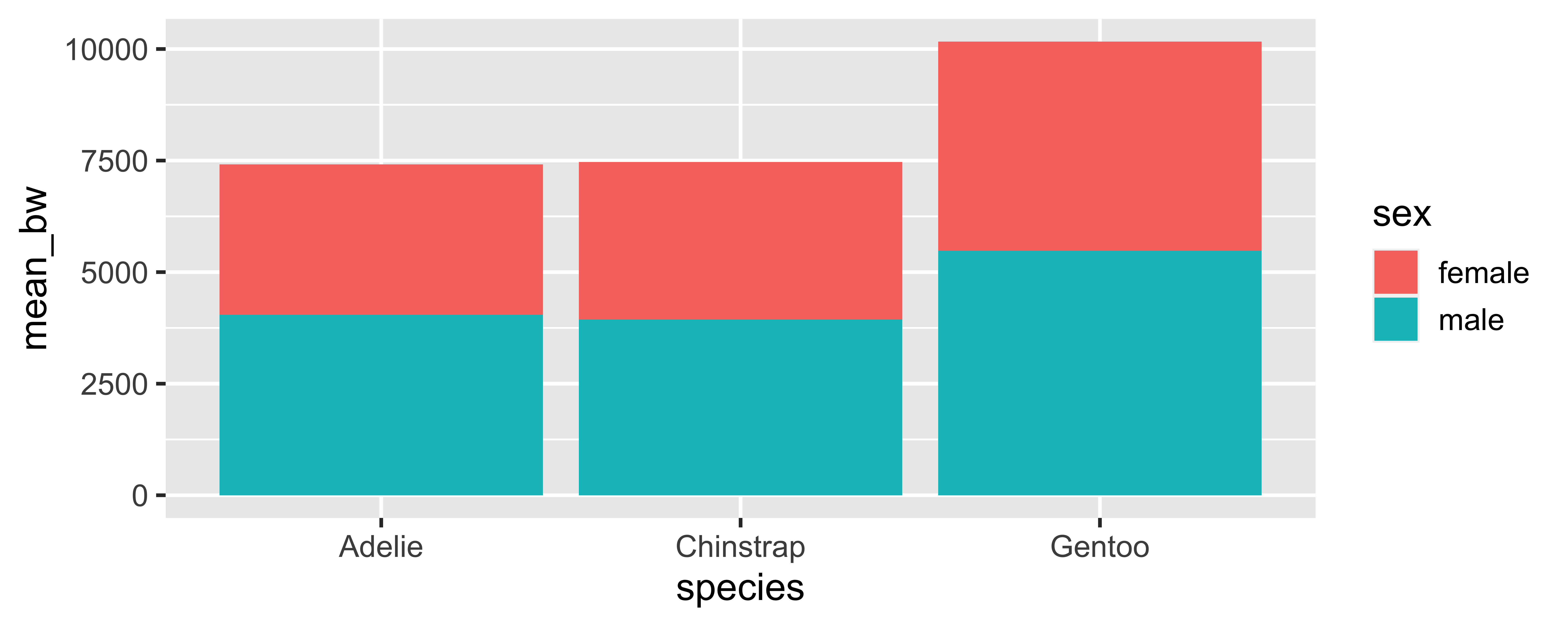
persistent grouping - handle with .groups

Remember our “typical tidyverse pipeline”? Why did we set .groups = "drop" in summarize()?

penguins |>
  drop_na(sex, body_mass_g) |>
  group_by(species, sex) |>
  summarize(mean_bw = mean(body_mass_g), .groups = "drop") |>
  ggplot(aes(x = species, y = mean_bw, fill = sex)) +
  geom_col(position = "dodge")

persistent grouping - message

What if we don’t set it? Why does summarize() emit a message even though the result doesn’t change?

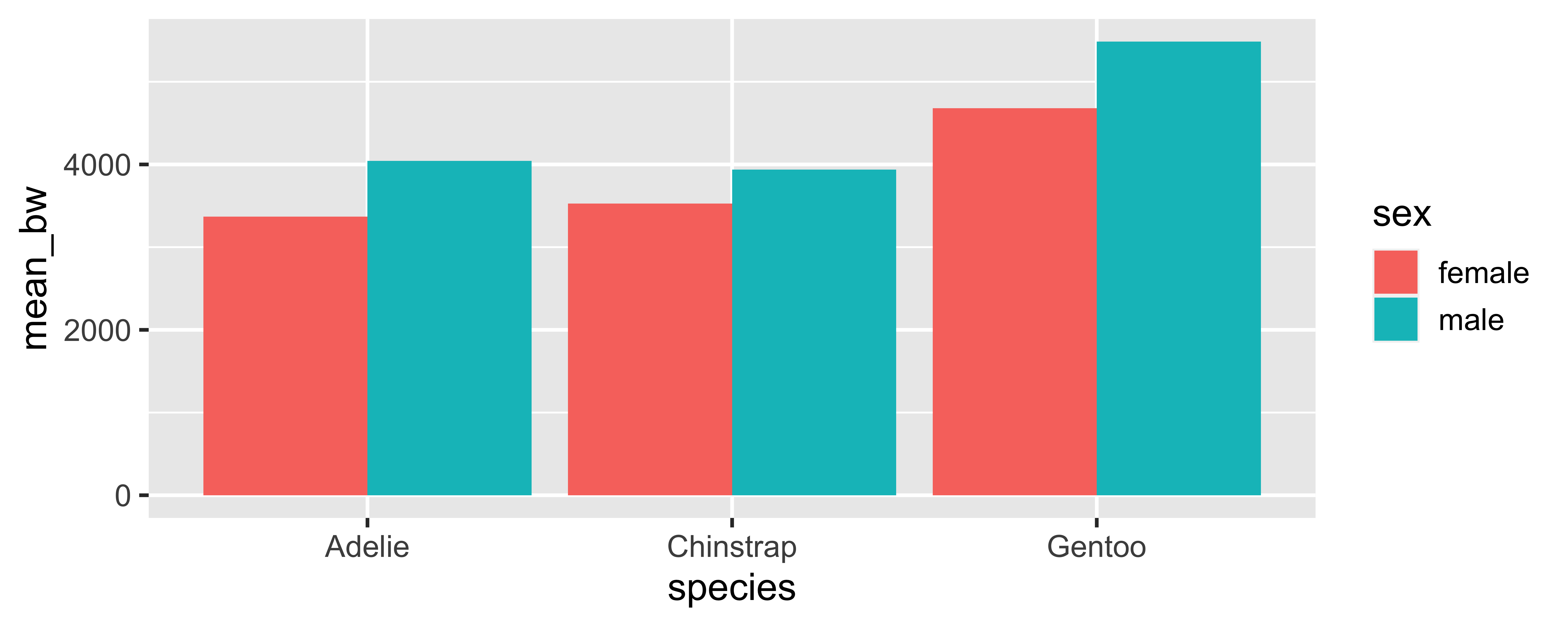
penguins |>
  drop_na(sex, body_mass_g) |>
  group_by(species, sex) |>
  summarize(mean_bw = mean(body_mass_g)) |>
  ggplot(aes(x = species, y = mean_bw, fill = sex)) +
  geom_col(position = "dodge")

`summarise()` has grouped output by 'species'. You can override
using the `.groups` argument.

persistent grouping - downstream effects

persistent groups:

penguins |>
  drop_na(sex, body_mass_g) |>
  group_by(species, sex) |>
  summarize(mean_bw = mean(body_mass_g)) |>
  slice_head(n = 1)

`summarise()` has grouped output by 'species'. You can override
using the `.groups` argument.

# A tibble: 3 × 3
# Groups:   species [3]
  species   sex    mean_bw
  <fct>     <fct>    <dbl>
1 Adelie    female   3369.
2 Chinstrap female   3527.
3 Gentoo    female   4680.

dropped groups:

penguins |>
  drop_na(sex, body_mass_g) |>
  group_by(species, sex) |>
  summarize(mean_bw = mean(body_mass_g), .groups = "drop") |>
  slice_head(n = 1)

# A tibble: 1 × 3
  species sex    mean_bw
  <fct>   <fct>    <dbl>
1 Adelie  female   3369.

persistent grouping - downstream effects

persistent groups:

penguins |>
  drop_na(sex, body_mass_g) |>
  group_by(species, sex) |>
  summarize(mean_bw = mean(body_mass_g)) |>
  gt::gt()

`summarise()` has grouped output by 'species'. You can override
using the `.groups` argument.

sex	mean_bw
Adelie
female	3368.836
male	4043.493
Chinstrap
female	3527.206
male	3938.971
Gentoo
female	4679.741
male	5484.836

dropped groups:

penguins |>
  drop_na(sex, body_mass_g) |>
  group_by(species, sex) |>
  summarize(mean_bw = mean(body_mass_g), .groups = "drop") |>
  gt::gt()

species	sex	mean_bw
Adelie	female	3368.836
Adelie	male	4043.493
Chinstrap	female	3527.206
Chinstrap	male	3938.971
Gentoo	female	4679.741
Gentoo	male	5484.836

handling grouping - option 1

What we’ve already seen, explicitly selecting what to do with groups with .groups:

drop groups:

penguins |>
  drop_na(sex, body_mass_g) |>
  group_by(species, sex) |>
  summarize(
    mean_bw = mean(body_mass_g), 
    .groups = "drop"
  )

# A tibble: 6 × 3
  species   sex    mean_bw
  <fct>     <fct>    <dbl>
1 Adelie    female   3369.
2 Adelie    male     4043.
3 Chinstrap female   3527.
4 Chinstrap male     3939.
5 Gentoo    female   4680.
6 Gentoo    male     5485.

keep groups:

penguins |>
  drop_na(sex, body_mass_g) |>
  group_by(species, sex) |>
  summarize(
    mean_bw = mean(body_mass_g), 
    .groups = "keep"
  )

# A tibble: 6 × 3
# Groups:   species, sex [6]
  species   sex    mean_bw
  <fct>     <fct>    <dbl>
1 Adelie    female   3369.
2 Adelie    male     4043.
3 Chinstrap female   3527.
4 Chinstrap male     3939.
5 Gentoo    female   4680.
6 Gentoo    male     5485.

handling grouping - option 2

Using per-operation grouping with .by:

group by 1 var:

penguins |>
  drop_na(sex, body_mass_g) |>
  summarize(
    mean_bw = mean(body_mass_g), 
    .by = species
  )

# A tibble: 3 × 2
  species   mean_bw
  <fct>       <dbl>
1 Adelie      3706.
2 Gentoo      5092.
3 Chinstrap   3733.

group by 2+ vars:

penguins |>
  drop_na(sex, body_mass_g) |>
  summarize(
    mean_bw = mean(body_mass_g), 
    .by = c(species, sex)
  )

# A tibble: 6 × 3
  species   sex    mean_bw
  <fct>     <fct>    <dbl>
1 Adelie    male     4043.
2 Adelie    female   3369.
3 Gentoo    female   4680.
4 Gentoo    male     5485.
5 Chinstrap female   3527.
6 Chinstrap male     3939.

group_by() vs. .by

• group_by() is not superseded and not going away, .by is an alternative if you want per-operation grouping.

• Some verbs take by instead of .by as an argument 😞, but they come with informative errors 🙂

• .by always returns an ungrouped data frame

• You can’t create variables on the fly in .by, you must create them earlier in your pipeline, e.g., unlike df |> group_by(month = floor_date(date, "month"))

• .by doesn’t sort grouping keys, group_by() always sorts keys in ascending order, which affects the results of verbs like summarise(), e.g., see the species orders in the two previous slides

teaching tip

Choose one grouping method and stick to it

It doesn’t matter whether you use group_by() (followed by .groups, where needed) or .by.

• For new learners, pick one and stick to it.
• For more experienced learners, particularly those learning to design their own functions and packages, it can be interesting to go through the differences and evolution.

quality of life improvements

for case_when() and if_else():

• all else denoted by .default for case_when()
• less strict about value type for both

previously

df |>
  mutate(
    x = case_when(
      <condition 1> ~ "value 1",
      <condition 2> ~ "value 2",
      <condition 3> ~ "value 3",
      TRUE          ~ NA_character_
    )
  )

now - optionally

df |>
  mutate(
    x = case_when(
      <condition 1> ~ "value 1",
      <condition 2> ~ "value 2",
      <condition 3> ~ "value 3",
      .default = NA
    )
  )

setup: penguin_quantiles

penguins |>
  reframe(bm_cat = quantile(body_mass_g, c(0.25, 0.75), na.rm = TRUE))

# A tibble: 2 × 1
  bm_cat
   <dbl>
1   3550
2   4750

case_when()

penguins |>
  mutate(
    bm_cat = case_when(
      is.na(body_mass_g) ~ NA,
      body_mass_g < 3550 ~ "Small",
      between(body_mass_g, 3550, 4750) ~ "Medium",
      .default = "Large"
    )
  ) |>
  relocate(body_mass_g, bm_cat)

# A tibble: 344 × 9
  body_mass_g bm_cat species island  bill_length_mm bill_depth_mm
        <int> <chr>  <fct>   <fct>            <dbl>         <dbl>
1        3750 Medium Adelie  Torger…           39.1          18.7
2        3800 Medium Adelie  Torger…           39.5          17.4
3        3250 Small  Adelie  Torger…           40.3          18  
4          NA <NA>   Adelie  Torger…           NA            NA  
5        3450 Small  Adelie  Torger…           36.7          19.3
6        3650 Medium Adelie  Torger…           39.3          20.6
# ℹ 338 more rows
# ℹ 3 more variables: flipper_length_mm <int>, sex <fct>,
#   year <int>

if_else()

penguins |>
  mutate(
    bm_unit = if_else(!is.na(body_mass_g), paste(body_mass_g, "g"), NA)
  ) |>
  relocate(body_mass_g, bm_unit)

# A tibble: 344 × 9
  body_mass_g bm_unit species island bill_length_mm bill_depth_mm
        <int> <chr>   <fct>   <fct>           <dbl>         <dbl>
1        3750 3750 g  Adelie  Torge…           39.1          18.7
2        3800 3800 g  Adelie  Torge…           39.5          17.4
3        3250 3250 g  Adelie  Torge…           40.3          18  
4          NA <NA>    Adelie  Torge…           NA            NA  
5        3450 3450 g  Adelie  Torge…           36.7          19.3
6        3650 3650 g  Adelie  Torge…           39.3          20.6
# ℹ 338 more rows
# ℹ 3 more variables: flipper_length_mm <int>, sex <fct>,
#   year <int>

teaching tip

It’s a blessing to not have to introduce NA_character_ and friends

Especially not having to introduce it as early as if_else() and case_when(). Cherish it!

Different types of NAs are a good topic for a course on R as a programming language, statistical computing, etc. but not necessary for an intro course.

and more…

• Further simplify your case_when() statements with case_match()
• Selecting columns inside a function like mutate() or summarize() with pick()
• Reproducibility and performance updates to arrange()
• Read more at https://www.tidyverse.org/tags/dplyr-1-1-0/

tidyr 1.3.0

new separate_*() functions

that supersede extract(), separate(), and separate_rows() because they have more consistent names and arguments, have better performance, and provide a new approach for handling problems:

	MAKE COLUMNS	MAKE ROWS
Separate with delimiter	separate_wider_delim()	separate_longer_delim()
Separate by position	separate_wider_position()	separate_longer_position()
Separate with regular expression	separate_wider_regex()

setup: three_penguin_descriptions

three_penguin_descriptions <- tribble(
  ~id, ~description,
  1,   "Species: Adelie, Island - Torgersen",
  2,   "Species: Gentoo, Island - Biscoe",
  3,   "Species: Chinstrap, Island - Dream",
)

three_penguin_descriptions

# A tibble: 3 × 2
     id description                        
  <dbl> <chr>                              
1     1 Species: Adelie, Island - Torgersen
2     2 Species: Gentoo, Island - Biscoe   
3     3 Species: Chinstrap, Island - Dream 

separate_wider_delim()

three_penguin_descriptions |>
  separate_wider_delim(
    cols = description,
    delim = ", ",
    names = c("species", "island")
  )

# A tibble: 3 × 3
     id species            island            
  <dbl> <chr>              <chr>             
1     1 Species: Adelie    Island - Torgersen
2     2 Species: Gentoo    Island - Biscoe   
3     3 Species: Chinstrap Island - Dream    

separate_wider_regex()

If you’re into that sort of thing…

three_penguin_descriptions |>
  separate_wider_regex(
    cols = description,
    patterns = c(
      "Species: ", species = "[^,]+", 
      ", ", 
      "Island - ", island = ".*"
    )
  )

# A tibble: 3 × 3
     id species   island   
  <dbl> <chr>     <chr>    
1     1 Adelie    Torgersen
2     2 Gentoo    Biscoe   
3     3 Chinstrap Dream    

enhanced reporting when things fail

previously

separate(
  data,
  col,
  into,
  sep = "[^[:alnum:]]+",
  remove = TRUE,
  convert = FALSE,
  extra = "warn",
  fill = "warn",
  ...
)

now

separate_wider_*(
  data,
  cols,
  <depends on method to separate>,
  ...,
  names = NULL,
  names_sep = NULL,
  names_repair = "check_unique",
  too_few = c("error", "debug", "align_start", "align_end"),
  too_many = c("error", "debug", "drop", "merge"),
  cols_remove = TRUE  
)

teaching tip

Excel text-to-column users are used to different approaches to “separate”

If teaching folks coming from doing data manipulation in spreadsheets, leverage that to motivate different types of separate_*() functions, and show the benefits of programming over point-and-click software for more advanced operations like separating longer and separating with regular expressions.

ggplot2 3.4.0

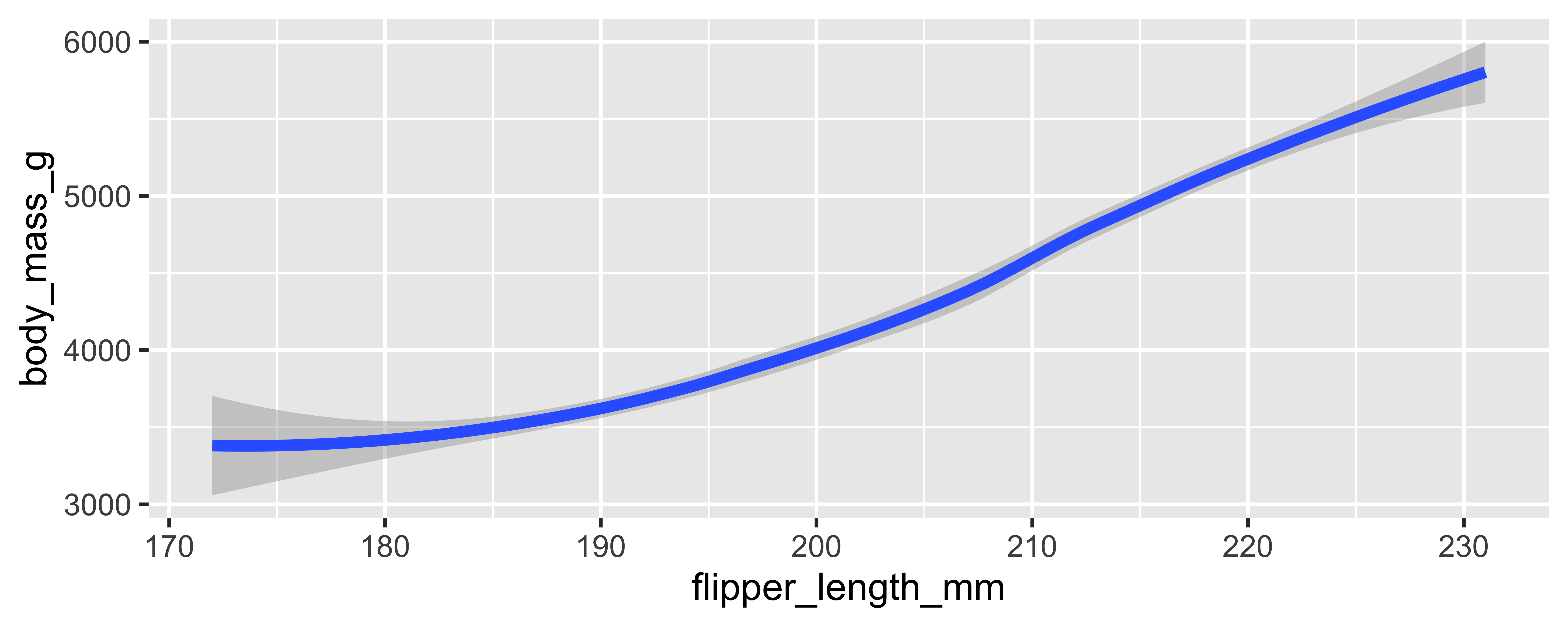
linewidth

previously

penguins |>
  drop_na() |>
  ggplot(
    aes(x = flipper_length_mm, y = body_mass_g)
  ) +
  geom_smooth(size = 2)

Warning: Using `size` aesthetic for lines was deprecated in ggplot2
3.4.0.
ℹ Please use `linewidth` instead.

now

penguins |>
  drop_na() |>
  ggplot(
    aes(x = flipper_length_mm, y = body_mass_g)
  ) +
  geom_smooth(linewidth = 2)

teaching tip

Check the output of your old teaching materials thoroughly

To not make a fool of yourself when teaching 🤣

and more…

other tidyverse updates

• Better stringr and tidyr alignment
• Ability to distinguish between NA in levels vs. NA in values in forcats
• New (more straightforward to learn/teach!) API for rvest
• Shorter, more readable, and (in some cases) faster SQL queries in dbplyr
• and more …

keeping up with the tidyverse

If you are interested in closely keeping up with updates in the tidyverse, the Tidyverse blog is the best place to read!

other tidyverse adjacent developments

The Tidyverse blog is also a great place to keep up with

• tidymodels updates

• and the magic that is webR! ✨

learn more

For a comprehensive overview of data science with R and the tidyverse, read the recently updated, and very soon to be available in paperback, R for Data Science, 2nd Edition.

thank you!

🔗 https://mine.quarto.pub/tidyverse-2023

💻 https://github.com/mine-cetinkaya-rundel/tidyverse-2023

References

Packages

• tidyverse: Wickham H, Averick M, Bryan J, Chang W, McGowan LD, François R, Grolemund G, Hayes A, Henry L, Hester J, Kuhn M, Pedersen TL, Miller E, Bache SM, Müller K, Ooms J, Robinson D, Seidel DP, Spinu V, Takahashi K, Vaughan D, Wilke C, Woo K, Yutani H (2019). “Welcome to the tidyverse.” Journal of Open Source Software, 4(43), 1686. doi:10.21105/joss.01686 https://doi.org/10.21105/joss.01686.

• palmerpenguins: Horst AM, Hill AP, Gorman KB (2020). palmerpenguins: Palmer Archipelago (Antarctica) penguin data. R package version 0.1.0. https://allisonhorst.github.io/palmerpenguins/. doi: 10.5281/zenodo.3960218.

• conflicted: Wickham H (2023). conflicted: An Alternative Conflict Resolution Strategy. R package version 1.2.0, https://CRAN.R-project.org/package=conflicted.

• gt: Iannone R, Cheng J, Schloerke B, Hughes E, Lauer A, Seo J (2023). gt: Easily Create Presentation-Ready Display Tables. R package version 0.9.0, https://CRAN.R-project.org/package=gt.