03:00
Documents
ASA Traveling Course: From R Markdown to Quarto
Dr. Mine Çetinkaya-Rundel
Duke University + Posit
2023-04-28
Anatomy of a Quarto document
Components
Metadata: YAML
Text: Markdown
Code: Executed via
knitrorjupyter
Weave it all together, and you have beautiful, powerful, and useful outputs!
Literate programming
Literate programming is writing out the program logic in a human language with included (separated by a primitive markup) code snippets and macros.
Metadata
YAML
“Yet Another Markup Language” or “YAML Ain’t Markup Language” is used to provide document level metadata.
Output options
Output option arguments
Indentation matters!
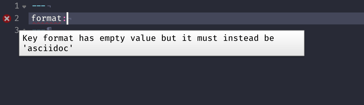
YAML validation
- Invalid: No space after
:
- Invalid: Read as missing
- Valid, but needs next object
YAML validation
There are multiple ways of formatting valid YAML:
- Valid: There’s a space after
:
- Valid: There are 2 spaces a new line and no trailing
:
- Valid:
format: htmlwith selections made with proper indentation
Why YAML?
To avoid manually typing out all the options, every time when rendering via the CLI:
Quarto linting
Lint, or a linter, is a static code analysis tool used to flag programming errors, bugs, stylistic errors and suspicious constructs.
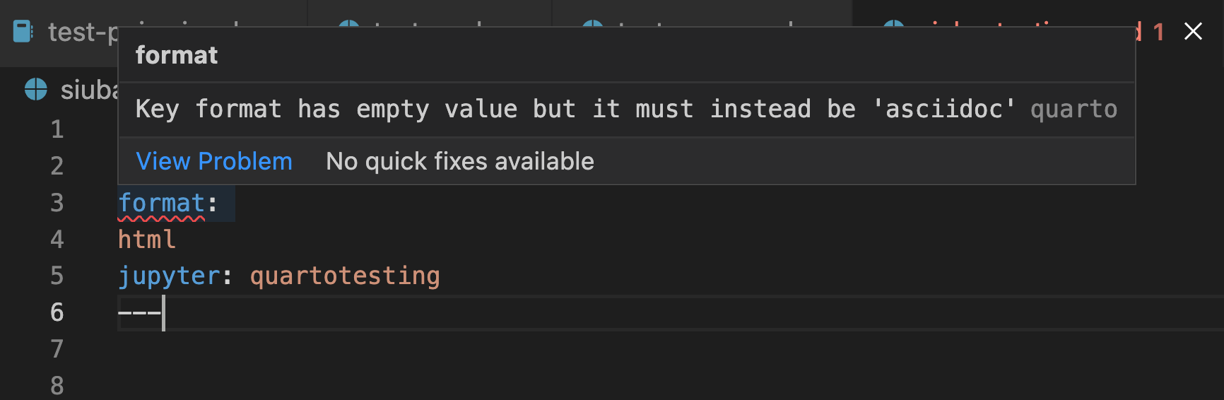
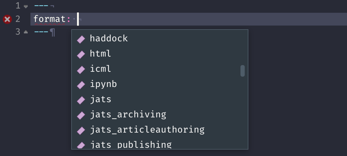
Quarto YAML Intelligence
RStudio + VSCode provide rich tab-completion - start a word and tab to complete, or Ctrl + space to see all available options.
Your turn
- Open
hello-penguins.qmdin RStudio. - Try
Ctrl + spaceto see the available YAML options. - Try out the tab-completion of any options you remember.
- You can use the HTML reference as needed.
List of valid YAML fields
Many YAML fields are common across various outputs
But also each output type has its own set of valid YAML fields and options
Definitive list: quarto.org/docs/reference/formats/html
Text
Text Formatting
| Markdown Syntax | Output |
|---|---|
|
italics and bold |
|
superscript2 / subscript2 |
|
|
|
verbatim code |
Headings
| Markdown Syntax | Output |
|---|---|
|
Header 1 |
|
Header 2 |
|
Header 3 |
|
Header 4 |
|
Header 5 |
|
Header 6 |
Links
There are several types of “links” or hyperlinks.
Markdown
Output
You can embed named hyperlinks, direct urls like https://quarto.org/, and links to other places in the document. The syntax is similar for embedding an inline image:  .
.
Lists
Unordered list:
Output
-   unordered list
    -   sub-item 1
    -   sub-item 1
        -   sub-sub-item 1
- sub-item 1
Ordered list:
Quotes
Markdown:
> Let us change our traditional attitude to the construction of programs: Instead of imagining that our main task is to instruct a computer what to do, let us concentrate rather on explaining to human beings what we want a computer to do.
> - Donald Knuth, Literate Programming
Output:
Let us change our traditional attitude to the construction of programs: Instead of imagining that our main task is to instruct a computer what to do, let us concentrate rather on explaining to human beings what we want a computer to do. - Donald Knuth, Literate Programming
Divs and spans
Pandoc, and therefore Quarto, can parse “fenced div blocks”:
- You can think of a
:::div as a HTML<div>but it can also apply in specific situations to content in PDF:
This content can be styled with a border
Divs with pre-defined classes
These can often apply between formats:
Your turn
- Open
markdown-syntax.qmdin RStudio. - Follow the instructions in the document, then exchange one new thing you’ve learned with your neighbor.
05:00
Callouts
::: callout-note
Note that there are five types of callouts, including:
`note`, `tip`, `warning`, `caution`, and `important`.
:::
Note
Note that there are five types of callouts, including: note, tip, warning, caution, and important.
More callouts
Warning
Callouts provide a simple way to attract attention, for example, to this warning.
Important
Danger, callouts will really improve your writing.
Caution
Here is something under construction.
Caption
Tip with caption.
Your turn
- Open
callout-boxes.qmdand render the document. - Using the visual editor, change the type of the first callouts box and then re-render. Also play with the options to change its appearance.
- Add a caption to the second callout box.
- Make the third callout box collapsible. Then, switch over to the source editor to inspect the markdown code.
- Change the format to PDF and re-render.
03:00
Footnotes
Pandoc supports numbering and formatting footnotes.
Inline footnotes
Here is an inline note.^[Inlines notes are easier to write,
since you don't have to pick an identifier and move down to
type the note.]
Here is an inline note.1
Inline footnotes
Here is an footnore reference[^1]

[^1]: This can be easy in some situations when you have a really long note or
don't want to inline complex outputs.
Here is an footnote reference1
Notice in both situations that the footnote is placed at the bottom of the page in presentations, whereas in a document it would be hoverable or at the end of the document.
Code
Anatomy of a code chunk
- Has 3x backticks on each end
- Engine (
r) is indicated between curly braces{r} - Options stated with the
#|(hashpipe):#| option1: value
Code, who is it for?
- The way you display code is very different for different contexts.
- In a teaching scenario like today, I really want to display code.
- In a business, you may want to have a data-science facing output which displays the source code AND a stakeholder-facing output which hides the code.
Code
If you simply want code formatting but don’t want to execute the code:
- Option 1: Use 3x back ticks + the language
```r
```r
head(penguins)
```Showing and hiding code with echo
The
echooption shows the code when set totrueand hides it when set tofalse.If you want to both execute the code and return the full code including backticks (like in a teaching scenario)
echo: fencedis your friend!
Tables and figures
In reproducible reports and manuscripts, the most commonly included code outputs are tables and figures.
So they get their own special sections in our deep dive!
Tables
Markdown tables
Markdown:
| Right | Left | Default | Center |
|------:|:-----|---------|:------:|
|   12  |  12  |    12   |    12  |
|  123  |  123 |   123   |   123  |
|    1  |    1 |     1   |     1  |
Output:
| Right | Left | Default | Center |
|---|---|---|---|
| 12 | 12 | 12 | 12 |
| 123 | 123 | 123 | 123 |
| 1 | 1 | 1 | 1 |
Grid tables
Markdown:
+---------------+---------------+--------------------+
| Fruit         | Price         | Advantages         |
+===============+===============+====================+
| Bananas       | $1.34         | - built-in wrapper |
|               |               | - bright color     |
+---------------+---------------+--------------------+
| Oranges       | $2.10         | - cures scurvy     |
|               |               | - tasty            |
+---------------+---------------+--------------------+

: Sample grid table.
Grid tables
Output:
| Fruit | Price | Advantages |
|---|---|---|
| Bananas | $1.34 |
|
| Oranges | $2.10 |
|
Grid tables: Alignment
- Alignments can be specified as with pipe tables, by putting colons at the boundaries of the separator line after the header:
+---------------+---------------+--------------------+
| Right         | Left          | Centered           |
+==============:+:==============+:==================:+
| Bananas       | $1.34         | built-in wrapper   |
+---------------+---------------+--------------------+- For headerless tables, the colons go on the top line instead:
+--------------:+:--------------+:------------------:+
| Right         | Left          | Centered           |
+---------------+---------------+--------------------+
Grid tables: Authoring
Note that grid tables are quite awkward to write with a plain text editor because unlike pipe tables, the column indicators must align.
The Visual Editor can assist in making these tables!
Tables from code
The knitr package can turn data frames into tables with knitr::kable():
| species | island | bill_length_mm | bill_depth_mm | flipper_length_mm | body_mass_g | sex | year |
|---|---|---|---|---|---|---|---|
| Adelie | Torgersen | 39.1 | 18.7 | 181 | 3750 | male | 2007 |
| Adelie | Torgersen | 39.5 | 17.4 | 186 | 3800 | female | 2007 |
| Adelie | Torgersen | 40.3 | 18.0 | 195 | 3250 | female | 2007 |
| Adelie | Torgersen | NA | NA | NA | NA | NA | 2007 |
| Adelie | Torgersen | 36.7 | 19.3 | 193 | 3450 | female | 2007 |
| Adelie | Torgersen | 39.3 | 20.6 | 190 | 3650 | male | 2007 |
Tables from code
If you want fancier tables, try the gt package and all that it offers!
| species | island | bill_length_mm | bill_depth_mm | flipper_length_mm | body_mass_g | sex | year |
|---|---|---|---|---|---|---|---|
| Adelie | Torgersen | 39.1 | 18.7 | 181 | 3750 | male | 2007 |
| Adelie | Torgersen | 39.5 | 17.4 | 186 | 3800 | female | 2007 |
| Adelie | Torgersen | 40.3 | 18.0 | 195 | 3250 | female | 2007 |
| Adelie | Torgersen | NA | NA | NA | NA | NA | 2007 |
| Adelie | Torgersen | 36.7 | 19.3 | 193 | 3450 | female | 2007 |
| Adelie | Torgersen | 39.3 | 20.6 | 190 | 3650 | male | 2007 |
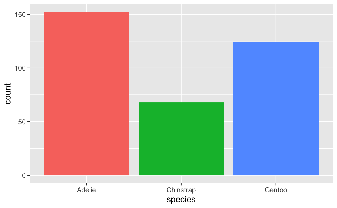
Figures
Markdown figures
Penguins playing with a Quarto ball
Markdown figures with options
{fig-align="left"}
{fig-align="right" fig-alt="Illustration of two penguins playing with a Quarto ball."}
Subfigures
Markdown:
::: {#fig-penguins layout-ncol=2}
{#fig-blue width="250px"}
{#fig-orange width="250px"}
Two penguins
:::Subfigures
Output:


Figure divs
Markdown:
Figure divs
Output:
Last paragraph in the div block is used as the figure caption.
Finding the figures to include
In places like markdown, YAML, or the command line/shell/terminal, you’ll need to use absolute or relative file paths:
- Absolute = BAD:
"/Users/mine/quarto-asa-nebraska"- Whose computer will this work on?
Relative = BETTER:
"../= up one directory,../../= up two directories, etc./..or/= start fromrootdirectory of your current computer
Figures with code
Referencing paths in R code
Use the here package to reference the project root, as here::here() always starts at the top-level directory of a .Rproj:
[1] "/Users/mine/Desktop/Workshops/quarto/quarto-asa-nebraska" [1] "_extensions" "_freeze"
[3] "_publish.yml" "_quarto.yml"
[5] "_site" "1-hello-quarto"
[7] "2-documents" "3-presentations"
[9] "4-websites" "exercises"
[11] "images" "index.html"
[13] "index.qmd" "LICENSE.html"
[15] "LICENSE.md" "pre-work.html"
[17] "pre-work.qmd" "quarto-asa-nebraska.Rproj"
[19] "README.md" "site_libs"
[21] "style" Figures from code
Cross references
Cross references
Help readers to navigate your document with numbered references and hyperlinks to entities like figures and tables.
Cross referencing steps:
- Add a caption to your figure or table.
- Give an id to your figure or table, starting with
fig-ortbl-. - Refer to it with
@fig-...or@tbl-....
Figure cross references
The presence of the caption (Blue penguin) and label (#fig-blue-penguin) make this figure referenceable:
Markdown:
Table cross references
The presence of the caption (A few penguins) and label (#tbl-penguins) make this table referenceable:
Markdown:
Output:
See Table 1 for data on a few penguins.
| species | island | bill_length_mm | bill_depth_mm | flipper_length_mm | body_mass_g | sex | year |
|---|---|---|---|---|---|---|---|
| Adelie | Torgersen | 39.1 | 18.7 | 181 | 3750 | male | 2007 |
| Adelie | Torgersen | 39.5 | 17.4 | 186 | 3800 | female | 2007 |
| Adelie | Torgersen | 40.3 | 18.0 | 195 | 3250 | female | 2007 |
| Adelie | Torgersen | NA | NA | NA | NA | NA | 2007 |
| Adelie | Torgersen | 36.7 | 19.3 | 193 | 3450 | female | 2007 |
| Adelie | Torgersen | 39.3 | 20.6 | 190 | 3650 | male | 2007 |
Your turn
- Open
tables-figures.qmd. - Follow the instructions in the document, then exchange one new thing you’ve learned with your neighbor.
10:00
Wrap up
Questions
Any questions / anything you’d like to review before we wrap up this module?